BE/B.Tech | Signal and System | For E.C.E. & E.I.E Second Year, III Semester IMP QnA.

Q1. Explain the system and its classification.

Definition of a System:

A system can be defined as a functional block that takes one or more input signals and produces one or more output signals. The input signals represent the information or stimuli provided to the system, while the output signals represent the response or transformation of the input signals by the system.

Classification of Systems:

Systems can be classified based on various criteria, including their properties, behavior, and mathematical representations. Here are some common classifications of systems:

1. Based on Input and Output Nature:
• Continuous-Time Systems: These systems process signals that are defined for all real numbers. They operate on continuous-time signals.
• Discrete-Time Systems: These systems process signals that are defined only at discrete points in time. They operate on discrete-time signals.
2. Based on Linearity and Time-Invariance:
• Linear Systems: Systems that satisfy the properties of superposition and homogeneity are considered linear.
• Time-Invariant Systems: Systems whose properties and behavior do not change over time are considered time-invariant.
3. Based on Memory:
• Memoryless Systems: Systems whose output at any given time depends only on the input at that same time are considered memoryless.
• Memory Systems: Systems whose output depends on the current and past values of the input are considered memory systems.
4. Based on Causality:
• Causal Systems: Systems whose output depends only on the current and past values of the input (i.e., they cannot anticipate future inputs).
• Non-causal Systems: Systems whose output depends on future as well as past and current values of the input.
5. Based on Stability:
• Stable Systems: Systems in which bounded inputs result in bounded outputs.
• Unstable Systems: Systems in which bounded inputs may result in unbounded outputs.

Q2. Explain even and odd signal

Even Signal:

• An even signal is symmetric about the vertical axis or the y-axis.
• Mathematically, a signal x(t) is even if it satisfies the property: x(t)=x(−t) for all t in its domain.
• In the discrete-time domain, a signal x[n] is even if it satisfies the property: = x[n]= x[−n] for all n.
• An even signal's plot appears identical when reflected across the y-axis.
• Example: The cosine function is an example of an even signal.

Odd Signal:

• An odd signal is symmetric about the origin (0,0) or the point of intersection of the signal with the y-axis.
• Mathematically, a signal x(t) is odd if it satisfies the property: = −x(−t) for all t in its domain.
• In the discrete-time domain, a signal x[n] is odd if it satisfies the property: x[n]=−x[−n] for all n.
• An odd signal's plot appears as its mirror image when reflected across the origin.
• Example: The sine function is an example of an odd signal.

Key Points:

• An even signal contains only cosine terms in its Fourier series representation.
• An odd signal contains only sine terms in its Fourier series representation.
• Some signals can be neither even nor odd, while some signals can be both.

Q3. What is an LTI system? How discrete time LTI system Differs from continuous time LTI system?

LTI System:

An LTI system is characterized by two main properties:

1. Linearity:
• A system is linear if it follows the principles of superposition and homogeneity.
• Superposition: The response to a sum of inputs equals the sum of responses to each individual input.
• Homogeneity: Scaling the input scales the output proportionally.
2. Time-Invariance:
• A system is time-invariant if its response does not change over time.
• This means that a time shift in the input signal results in the same time shift in the output signal.

Discrete-Time LTI System vs. Continuous-Time LTI System:

1. Discrete-Time LTI System:

• Discrete-time LTI systems operate on signals that are defined at discrete points in time.
• The input and output signals of these systems are sequences, usually represented by x[n] and y[n] respectively.
• The system's behavior is defined by linear constant-coefficient difference equations.
• The impulse response of a discrete-time LTI system is a sequence, denoted by h[n].
• Convolution in discrete time involves summing products of the input signal and the system's impulse response at different time shifts.

2. Continuous-Time LTI System:

• Continuous-time LTI systems operate on signals that are defined for all real numbers.
• The input and output signals are continuous-time functions, usually represented by x(t) and y(t) respectively.
• The system's behavior is described by linear constant-coefficient differential equations.
• The impulse response of a continuous-time LTI system is a function, denoted by h(t).
• Convolution in continuous time involves integrating the product of the input signal and the system's impulse response over all time shifts.

Differences:

1. Representation of Signals: Discrete-time systems deal with sequences, while continuous-time systems deal with functions.
2. Mathematical Representation: Discrete-time systems are described using difference equations, while continuous-time systems are described using differential equations.
3. Impulse Response: In discrete time, the impulse response is a sequence, while in continuous time, it is a function.
4. Convolution: The convolution operation is performed differently in discrete and continuous time due to the nature of the signals involved.

Q.4 Explain the Fourier transform. Also write any two properties of Fourier transform.

The Fourier Transform is a powerful mathematical tool used to decompose a signal into its constituent frequencies. It is widely used in various fields such as signal processing, communication systems, image processing, and more.

Fourier Transform:

The Fourier Transform of a signal is a mathematical operation that transforms a function of time (or space) into a function of frequency. It allows us to represent a signal in the frequency domain, where we can analyze its frequency content, amplitude, and phase characteristics.

For a continuous-time signal x(t), the Fourier Transform X(f) is defined as:

Where:

• x(t) is the input signal,
• X(f) is its Fourier Transform, and
• f represents frequency.

For a discrete-time signal x[n], the Discrete Fourier Transform (DFT) is used, which is a sampled version of the continuous Fourier Transform.

These properties make the Fourier Transform an invaluable tool for analyzing and manipulating signals in both time and frequency domains. It allows us to understand the frequency content of signals, filter out unwanted frequencies, and perform operations such as convolution and modulation.

 

Q.5 Define and explain casual and non-casual system.

Certainly! In the context of signal processing and systems theory, the terms "causal" and "non-causal" describe important characteristics of systems based on their response to input signals.

Causal System:

A causal system is one where the output of the system depends only on present and past values of the input signal, not future values. In other words, the system's response at any given time is determined solely by the input values up to that time.

Mathematically, for a continuous-time system, a system H(t) is causal if:

h(t)=0 for t<0

For a discrete-time system, a system H[n] is causal if:

h[n]=0 for n<0

In simpler terms, a causal system cannot "anticipate" or "predict" future input values when generating its output.

Non-Causal System:

Conversely, a non-causal system is one where the output at a given time depends on future as well as present and past values of the input signal. These systems exhibit behavior that violates the principle of causality.

Mathematically, for a continuous-time system, a system H(t) is non-causal if it has non-zero response for t<0.

For a discrete-time system, a system H[n] is non-causal if it has non-zero response for n<0.

Non-causal systems are often theoretical constructs and are not typically encountered in practical applications because they imply the ability to predict the future based on present and past observations.

Examples:

• Causal System: A simple low-pass filter where the output at any time depends only on the input signal values up to that time.
• Non-Causal System: A filter that tries to predict future values of a signal based on present and past values. Such a system would be non-causal, and in practical terms, it would be difficult to implement because it would require knowledge of future input values.

 

Q.6 state and prove sampling theorem

Statement of the Sampling Theorem:

The Sampling Theorem states that:

"A continuous-time signal x(t) can be perfectly reconstructed from its samples if and only if the sampling frequency fs​ is greater than twice the maximum frequency component f_max​ present in the signal, i.e. fs​>2f_max​."

Proof Sketch:

To prove the Sampling Theorem, let's consider a continuous-time signal x(t) with a bandwidth limited to f_max​ Hz.

1. Sampling Process:
• We sample the continuous-time signal x(t) at a rate of f_s​ samples per second to obtain the discrete-time signal x[n].
• The sampling rate f_s​ is measured in samples per second or Hz.
2. Reconstruction:
• According to the Nyquist-Shannon theorem, x(t) can be perfectly reconstructed from its samples if the sampling frequency f_s​ satisfies f_s ​>2f_max​.
3. Frequency Domain Analysis:
• In the frequency domain, the spectrum of x(t) is limited to f_max​ Hz.
• Due to the Nyquist criterion, the spectrum of the sampled signal x[n] repeats at intervals of f_s​ Hz.
4. Avoiding Aliasing:
• Aliasing occurs when frequencies above f_max​ fold back into the frequency range of interest during sampling, causing distortion.
• To avoid aliasing, f_s​ must be greater than twice f_max​, ensuring that the spectra of adjacent replicas do not overlap.
5. Perfect Reconstruction:
• With f_s​>2f_max​, the original signal x(t) can be perfectly reconstructed from its samples x[n] using interpolation techniques.

Q.7 Define ROC. State and explain properties of ROC.

Definition of ROC:

The Region of Convergence (ROC) is the set of values of the complex variable z for which the Z-transform of a discrete-time signal or system converges. In other words, it is the region in the complex plane where the Z-transform exists and is finite.

Properties of ROC:

1. ROC Must Include the Unit Circle (Discrete-Time Systems):
• For a causal and stable discrete-time system, the ROC must include the unit circle in the z-plane. This ensures convergence and stability of the system.
• If the system is anti-causal, the ROC lies outside the unit circle.
2. ROC Is Uniquely Determined:
• The ROC is uniquely determined by the properties of the discrete-time signal or system, including its causality, stability, and the nature of the Z-transform.
3. ROC Is Either Inside or Outside of Singularities:
• The ROC cannot include any poles of the Z-transform. It must be either inside or outside of the poles in the z-plane.
• If the ROC includes the outermost pole, it extends to infinity in that direction.
4. ROC Can Be Bounded or Unbounded:
• The ROC can be bounded (limited in extent) or unbounded (extending to infinity in one or more directions) depending on the properties of the signal or system.
5. ROC and Causality:
• For a causal system, the ROC is the region exterior to the outermost pole.
• For an anti-causal system, the ROC is the region interior to the innermost pole.
• For a two-sided system, the ROC is an annular region between the innermost and outermost poles.
6. ROC and System Stability:
• The ROC provides insights into the stability of the discrete-time system. Generally, a stable system has an ROC including the unit circle.

Q.8 Difference between power signal and energy signal.

Power Signal:

A power signal is a signal for which the total power is finite and nonzero. It is usually associated with continuous signals that are non-periodic or with discrete signals that have infinite duration. The power signal's power is spread out over time.

• Mathematical Definition: For a continuous-time signal x(t), it is a power signal if the integral of the squared magnitude of the signal over time is finite:

• Example: A sinusoidal signal with finite amplitude and frequency is a power signal.

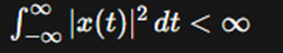
Energy Signal:

An energy signal is a signal for which the total energy is finite and nonzero. It is typically associated with signals that are either finite in duration or have a bounded amplitude.

• Mathematical Definition: For a continuous-time signal x(t), it is an energy signal if the integral of the squared magnitude of the signal over time is finite:

• Example: A finite-duration rectangular pulse signal with finite amplitude is an energy signal.

Differences:

1. Duration:
• Power signals may have infinite duration, while energy signals have finite duration.
2. Power vs. Energy:
• Power signals have finite power but potentially infinite energy.
• Energy signals have finite energy but potentially infinite power.
3. Application:
• Power signals are common in continuous communication channels where signals may be transmitted continuously.
• Energy signals are common in digital communication systems where signals are discrete and often have finite duration.
4. Analysis:
• Power signals are analyzed in terms of power spectral density and average power.
• Energy signals are analyzed in terms of energy spectral density and total energy.

 

Aspect	Power Signal	Energy Signal
Total Power	Finite and nonzero	Infinite or finite
Total Energy	Potentially infinite	Finite and nonzero
Duration	May be infinite	Finite
Mathematical Condition	(\int_{-\infty}^{\infty}	x(t)
Examples	Sinusoidal signals, periodic signals	Rectangular pulses, finite-duration signals
Application	Continuous communication channels	Digital communication systems
Analysis	Power spectral density, average power	Energy spectral density, total energy

Q.9 Determine the Z transform of the following signal x(n)= -naⁿ u (n-1).

Q.10 Find Z transform of the function an indicate the ROC x(n)=n(n+1) ⋅aⁿ ⋅u(n).

Q.11 Write short notes on Application of DTFT and Impulse response of DT-LTI system and its properties.

Application of DTFT (Discrete-Time Fourier Transform):

The Discrete-Time Fourier Transform (DTFT) is a fundamental tool in digital signal processing for analyzing the frequency content of discrete-time signals. Here are some key applications:

1. Frequency Analysis: DTFT helps in decomposing a discrete-time signal into its frequency components. This analysis is crucial for understanding the spectral characteristics of the signal.
2. Filter Design: DTFT aids in designing digital filters by providing insights into the frequency response of the system. Engineers can analyze the behavior of the filter in the frequency domain and optimize its performance based on desired specifications.
3. Spectrum Analysis: DTFT is used for spectrum analysis of discrete-time signals. It helps in identifying dominant frequencies, detecting harmonics, and analyzing periodic signals.
4. Signal Reconstruction: DTFT allows for signal reconstruction from its frequency components. By knowing the frequency content, one can reconstruct the original signal using inverse DTFT.
5. Fourier Transform Properties: Many properties of the continuous Fourier transform extend to the DTFT. These properties provide powerful tools for signal manipulation, including shifting, scaling, convolution, and modulation.

Impulse Response of DT-LTI System and its Properties:

A Discrete-Time Linear Time-Invariant (DT-LTI) system is characterized by its impulse response, which describes the system's behavior when subjected to a unit impulse input. Here are some key points about the impulse response of DT-LTI systems:

1. Definition: The impulse response h(n) of a DT-LTI system represents the output of the system when the input is a unit impulse δ(n).
2. Convolution Integral: The output of a DT-LTI system in response to any input signal x(n) can be obtained by convolving x(n) with the impulse response h(n). This convolution operation is fundamental in analyzing and understanding the behavior of DT-LTI systems.
3. Properties:
• Linearity: The impulse response of a DT-LTI system exhibits linearity. If h₁​(n) and h2​(n) are the impulse responses of two systems, then a₁​h₁​(n)+a₂​h_2​(n) is the impulse response of a linear combination a₁​h₁​(n)+a₂​h₂​(n).
• Time Invariance: The impulse response of a DT-LTI system is time-invariant. This means that if the input signal is delayed or advanced in time, the output is similarly delayed or advanced.
• Causality: Many practical systems are causal, meaning their impulse response is zero for negative time indices.
• Stability: DT-LTI systems are stable if the impulse response is absolutely summable, i.e.,
  
  
  
4. Frequency Response: The frequency response of a DT-LTI system, denoted by H(e^jω), is the Discrete-Time Fourier Transform (DTFT) of its impulse response. It provides insights into the system's behavior in the frequency domain and is crucial for filter design and analysis.

 

Q.12 Prove the properties of the time shifting in Z-transform.

The time-shifting property of the Z-transform states that if we shift a discrete-time signal x(n) by k units in time, the Z-transform of the shifted signal x(n−k) is given by z^−kX(z), where X(z) is the Z-transform of the original signal x(n). Let's prove this property formally:

Q.13 Parseval's Theorem.

Parseval's theorem, named after the French mathematician Marc-Antoine Parseval, is a fundamental result in signal processing and Fourier analysis. It relates the energy of a signal in the time domain to its energy in the frequency domain. The theorem holds for both continuous and discrete signals, and it provides an essential tool for signal analysis and system characterization.

Continuous-Time Case:

For a continuous-time signal x(t) with its Fourier transform X(f), Parseval's theorem states:

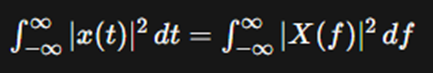
In words, the total energy of the signal x(t) over all time is equal to the total energy of its Fourier transform X(f) over all frequencies.

Discrete-Time Case:

For a discrete-time signal x[n] with its Discrete Fourier Transform (DFT) X[k], Parseval's theorem states:

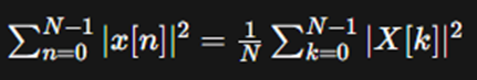
In words, the total energy of the discrete-time signal x[n] over all samples is equal to the sum of the squares of the magnitudes of its DFT coefficients X[k], normalized by the number of samples N.

Application and Importance:

• Energy Conservation: Parseval's theorem ensures that the total energy of a signal is conserved when transforming between the time and frequency domains.
• Signal Analysis: It provides a way to analyze the frequency content of a signal by examining its energy distribution in the frequency domain.
• System Characterization: Parseval's theorem is used to analyze the energy properties of signals processed by linear time-invariant (LTI) systems.
• Filter Design: Engineers use Parseval's theorem to design filters and ensure that the filter preserves the signal's energy content.

 

Q.14 Duality Theorem / Property of Fourier transform states and proved.

The Duality Theorem, also known as the Duality Property of the Fourier Transform, is a fundamental result in Fourier analysis that establishes a relationship between a function and its Fourier transform, as well as between the inverse Fourier transform of a function and its Fourier dual.